---
title: "Оглядовий аналіз та візуалізація даних у Python"
subtitle: "Лекція з практичними прикладами на Python"
author: "Богдан Красюк"
date: "2025-10-20"
lang: uk
categories: ["Лекції", "Аналітика даних"]
format:
html:
toc: true
toc-location: right
math: mathjax
toc-title: "План лекції"
toc-depth: 3
number-sections: true
code-fold: show
code-tools: true
smooth-scroll: true
execute:
echo: true
warning: false
message: false
---
## Презентація
<embed src="pdf/dataviz.pdf" width="100%" height="400px" type="application/pdf">
> 🎯 **Мета лекції.** Навчитися створювати інформативні графіки для **одновимірних**, **двовимірних** та **часових** даних у Python за допомогою **pandas** і **matplotlib**; опанувати базові патерни сторітелінгу, вибору типу графіка та підготовки даних до візуалізації.
## Підготовка середовища
```{python}
import pandas as pd
import numpy as np
import matplotlib.pyplot as plt
from pathlib import Path

# Розмір фігури за замовчуванням
plt.rcParams["figure.figsize"] = (8, 5)

# параметри відображення таблиць
pd.set_option("display.max_columns", None)
pd.set_option("display.max_rows", 20)

DATA_PATH = Path("data/input_data.csv")
print("Шлях до даних:", DATA_PATH.resolve())
```
## Завантаження та первинний огляд даних 🗂️
```{python}
# Завантаження CSV
df = pd.read_csv(DATA_PATH)

# Попередній перегляд
display(df.head(10))

# Розмір і типи
print("shape:", df.shape)
display(df.dtypes)

# Загальна інформація
df.info()
```
```{python}
# Описові статистики
# (include='all' для виводу і категоріальних полів)
display(df.describe(include="all").T)
```
## Підготовка до візуалізації: типи, дати/час, відсутні значення 🧰
```{python}
# Пошук потенційних колонок із датою/часом
date_like = [c for c in df.columns if any(k in c.lower() for k in ["date", "time", "dt", "timestamp"])]
for c in date_like:
    try:
        df[c] = pd.to_datetime(df[c], errors="raise", utc=False, dayfirst=True, infer_datetime_format=True)
        print(f"Стовпець перетворено у datetime: {c}")
    except Exception as e:
        print(f"Не вдалося перетворити {c} у datetime: {e}")

# Розділимо на числові/категоріальні для зручності
num_cols = df.select_dtypes(include=["number"]).columns.tolist()
cat_cols = df.select_dtypes(include=["object", "category", "bool"]).columns.tolist()
print("Числові:", num_cols[:8], ("..." if len(num_cols) > 8 else ""))
print("Категоріальні:", cat_cols[:8], ("..." if len(cat_cols) > 8 else ""))

# Оцінка пропусків
missing = df.isna().sum().sort_values(ascending=False)
display(missing.head(10))
```
> 💡 **Порада.** Перед побудовою графіків переконайтеся, що типи даних коректні (особливо дати) і пропуски або заповнені, або обробляються прямо у візуалізації (наприклад, через `dropna()`).
## Одновимірні розподіли 📊
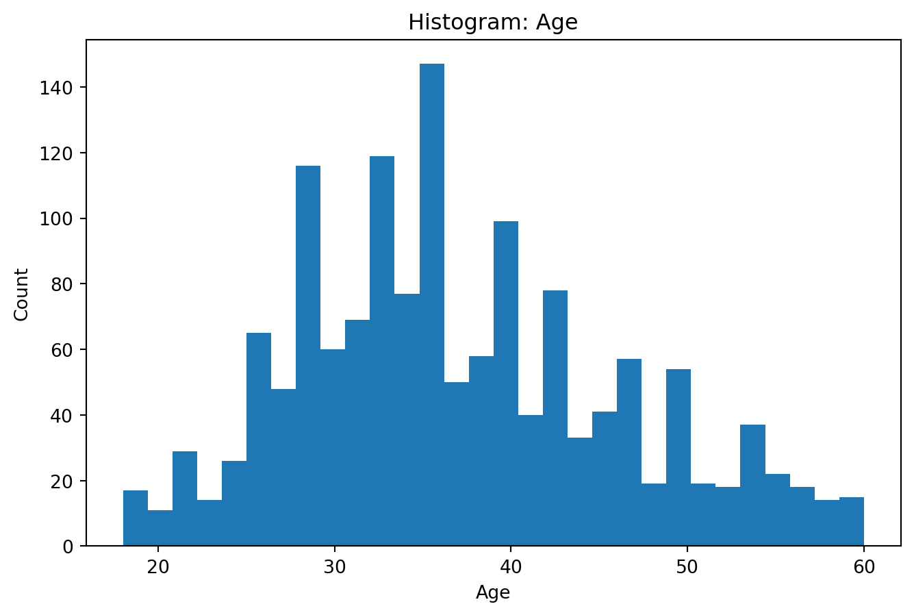
### Гістограма (кількісна змінна)
```{python}
# Оберемо першу числову колонку для прикладу
if num_cols:
    col = num_cols[0]
    series = df[col].dropna()

    plt.figure()
    plt.hist(series, bins=30)
    plt.title(f"Histogram: {col}")
    plt.xlabel(col); plt.ylabel("Count")
    plt.show()
else:
    print("Немає числових колонок для гістограми.")
```
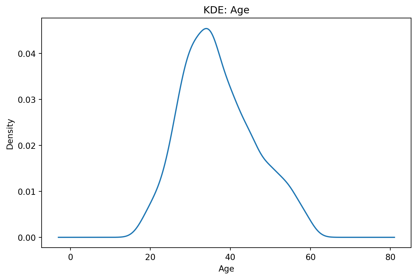
### Щільність розподілу (KDE) / емпірична CDF
```{python}
if num_cols:
col = num_cols[0]
series = df[col].dropna().sort_values()
# KDE через pandas
plt.figure()
series.plot(kind="kde")
plt.title(f"KDE: {col}")
plt.xlabel(col)
plt.show()
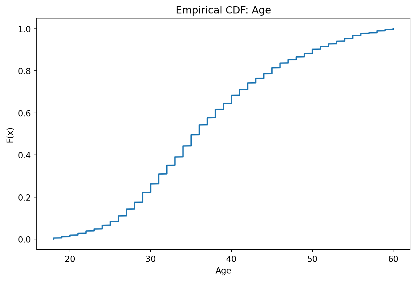
# Емпірична CDF
y = np.arange(1, len(series) + 1) / len(series)
plt.figure()
plt.plot(series.values, y)
plt.title(f"Empirical CDF: {col}")
plt.xlabel(col); plt.ylabel("F(x)")
plt.show()
```
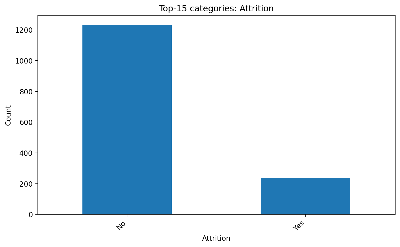
### Категоріальні частоти (Top-k барчарт)
```{python}
if cat_cols:
    c = cat_cols[0]
    counts = df[c].value_counts(dropna=False).head(15)

    plt.figure()
    counts.plot(kind="bar")
    plt.title(f"Top-15 categories: {c}")
    plt.xlabel(c); plt.ylabel("Count")
    plt.xticks(rotation=45, ha="right")
    plt.tight_layout()
    plt.show()
else:
    print("Немає категоріальних колонок для барчарту.")
```
## Двовимірні відношення 🔗
### Точкова діаграма (Scatter): кореляції та тренди
```{python}
# Візьмемо пару числових ознак із найбільшою за модулем кореляцією (крім діагоналі)
pair = None
if len(num_cols) >= 2:
    corr = df[num_cols].corr().abs()
    np.fill_diagonal(corr.values, 0.0)
    i, j = np.unravel_index(np.nanargmax(corr.values), corr.shape)
    xcol, ycol = num_cols[i], num_cols[j]
    pair = (xcol, ycol)

if pair:
    xcol, ycol = pair
    sub = df[[xcol, ycol]].dropna()

    plt.figure()
    plt.scatter(sub[xcol], sub[ycol], s=12, alpha=0.7)
    plt.title(f"Scatter: {xcol} vs {ycol}")
    plt.xlabel(xcol); plt.ylabel(ycol)
    plt.show()
else:
    print("Недостатньо числових ознак для побудови точкової діаграми.")
```
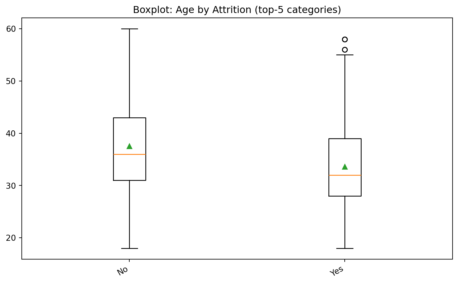
### Boxplot за категорією (ряд-до-ряду)
```{python}
# Boxplot однієї числової змінної за топ-5 категорій
if num_cols and cat_cols:
    vcol, gcol = num_cols[0], cat_cols[0]
    top_cats = df[gcol].value_counts().index[:5]
    data = [df.loc[df[gcol] == k, vcol].dropna().values for k in top_cats]

    plt.figure()
    plt.boxplot(data, labels=list(top_cats), showmeans=True)
    plt.title(f"Boxplot: {vcol} by {gcol} (top-5 categories)")
    plt.xticks(rotation=30, ha="right")
    plt.tight_layout()
    plt.show()
else:
    print("Потрібні принаймні 1 числова і 1 категоріальна змінні для boxplot.")
```
## Часові ряди ⏱️
```{python}
# Якщо є колонка datetime — побудуємо лінійний графік за місяцями для першої числової
dt_cols = df.select_dtypes(include=["datetime64[ns]", "datetime64[ns, UTC]"]).columns.tolist()
if dt_cols and num_cols:
    dtc, vcol = dt_cols[0], num_cols[0]
    ts = (
        df[[dtc, vcol]]
        .dropna()
        .sort_values(dtc)
        .set_index(dtc)[vcol]
        .resample("M")
        .mean()
    )

    plt.figure()
    plt.plot(ts.index, ts.values)
    plt.title(f"Time series (monthly mean): {vcol}")
    plt.xlabel("Date"); plt.ylabel(vcol)
    plt.tight_layout()
    plt.show()
else:
    print("Не знайдено datetime + числової колонки для часової візуалізації.")
```
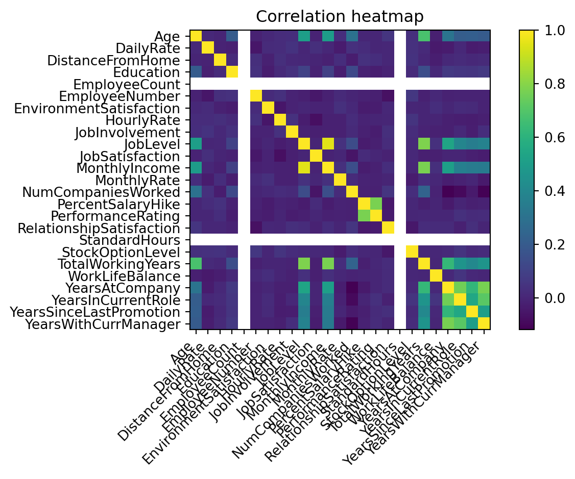
## Теплова карта кореляцій 🧭
```{python}
if len(num_cols) >= 2:
    corr = df[num_cols].corr()

    plt.figure()
    im = plt.imshow(corr.values, interpolation="nearest")
    plt.title("Correlation heatmap")
    plt.colorbar(im, fraction=0.046, pad=0.04)
    plt.xticks(range(len(num_cols)), num_cols, rotation=45, ha="right")
    plt.yticks(range(len(num_cols)), num_cols)
    plt.tight_layout()
    plt.show()
else:
    print("Недостатньо числових змінних для кореляційної теплокарти.")
```
## Сторітелінг і дизайн 🧩
- Починайте з **питання**: що саме хочемо побачити/довести?
- Вибирайте графік під **тип змінних** (кількісні/категоріальні/часові).
- Уникайте «діаграм-феєрверків»: **1 сюжет — 1 фігура**. Якщо огляд, робіть серію простих графіків.
- **Підписи осей, одиниці виміру, джерела** — обов’язково.
- Для порівнянь показуйте **однакові масштаби**, для великих діапазонів — лог-шкалу.
- Не перевантажуйте кольорами та сітками; акценти — через коментарі й підсумки.
## Міні‑завдання для самоперевірки 🧪
1. Оберіть 2 числові показники з максимальною кореляцією та побудуйте **scatter** з коротким висновком.
2. Для однієї ключової метрики побудуйте **histogram + KDE + CDF** і поясніть, як це впливає на бізнес‑рішення.
3. Створіть **boxplot** цієї метрики за 3–5 найчастіших категорій змінної групування і сформулюйте гіпотезу про відмінності.
4. Якщо є часова змінна — побудуйте **лінійний графік** агрегованого показника за тижнями/місяцями та прокоментуйте сезонність.
## Подальші кроки 🚀
- Додайте **контроль якості даних** у вигляді перевірок (діапазони, унікальність ключів, частка пропусків).
- Зробіть **функції/ноутбук** для повторного використання в інших проєктах.
- Підготуйте версію графіків для **звітів/дашбордів** (напр., Quarto + HTML).
---
### Ресурси для поглиблення
- Jupyter Notebook з лекції: [Pandas](notebooks/dataviz.ipynb)
- Лекційні матеріали «Оглядовий аналіз та візуалізація даних у Python».
- Kirthi Raman, *Mastering Python Data Visualization*, Packt.
---
:::: {.columns}
::: {.column width="20%"}
<img src="https://kleban.page/bc-2025/images/logo.png" alt="Лого" style="height: 70px;">
:::
::: {.column width="30%"}
<img src="https://kleban.page/bc-2025/images/eu-founded.png" alt="Лого" style="height: 100px;">
:::
::: {.column width="50%"}
Проєкт реалізується за підтримки **Європейського Союзу** в межах програми [Дім Європи](https://houseofeurope.org.ua/).
:::
::::